|
Chapter 3
Computer
Animation Technology
Computer animation provides a means of visually simulating the motion of a robotic system. Computer graphics might be thought of as the aspect of computer animation that actually displays the image of the robot system on the computer screen. If many robot images are displayed in rapid succession with the joint variables changed by a small amount each time, the robot image on the screen will appear to be moving in a continuous fashion. In order to produce a computer graphic simulation of the robot, it is necessary to communicate to the computer a description of the robot's visible surfaces. Besides the information necessary to produce a static image of the robot, a computer animation requires that the robot's kinematics be known as well. Since the computer animation will be used as a tool to visualize the robot in motion, it is important to understand the precision with which the computer displays the
image.
3.1 GRAPHICS
The graphical capabilities of the computer are used to display the image of the robot. Three-dimensional graphical presentation requires the use of three-dimensional transformations which may be represented as matrix operations. The description of the surface properties of the robot determines the appearance of the computer animation. Often times there is more than one surf ace in a single line of sight. In these cases it is necessary to do hidden surface removal so that only the surfaces nearest to the viewer are displayed. Because of the many operations that must be performed on each pixel that is to be displayed, such as rotation, translation and perspective transformations, a pipelined computer architecture is efficient for computer animation.
At the heart of three dimensional graphics are transformation and projection operations. These operations may be conveniently written in matrix form. The operation to translate an object while maintaining a constant orientation may be written as:
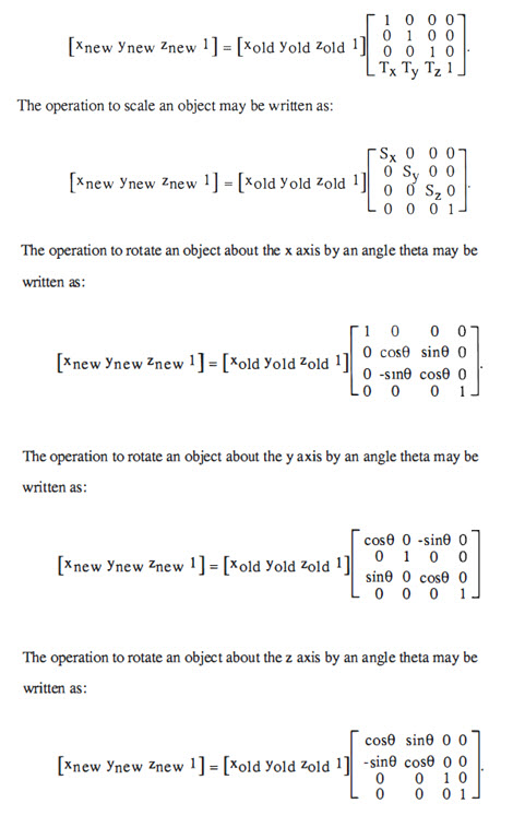
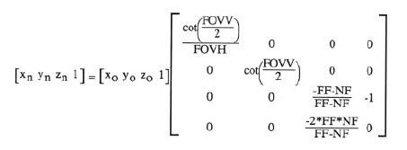
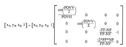
The projection transformations determine how a three-dimensional scene is projected onto the two-dimensional computer screen. In a perspective transformation it might be imagined that a three dimensional scene is being viewed through a pane of glass. If a line were drawn from every visible point on the scene back to the viewer's eye, and a dot were drawn on the pane of glass the exact same color as the points in the scene, then the two-dimensional drawing would appear to the viewer exactly the same as the three-dimensional scene. In order to define a scene for perspective transformation it is necessary to define where the pane of glass is; the near field, NF. It is necessary to know where the back of the scene is; the far field, FF. It is also necessary to know the field of view on the vertical, FOVV, and the field of view on the horizontal, FOVH. Using this terminology, the perspective projection may be written as:
|
|
A simpler and computationally faster type of projection operation is the orthographic transformation. The orthographic projection is orthogonal and, unlike the perspective projection, objects do not appear to get larger as they get closer to the viewer. A box shaped enclosure may be utilized in order to define an orthographic projection. It is necessary to define the front, back, top, bottom, left and right boundaries of the box. The orthographic projection operation may then be written as:
|
|
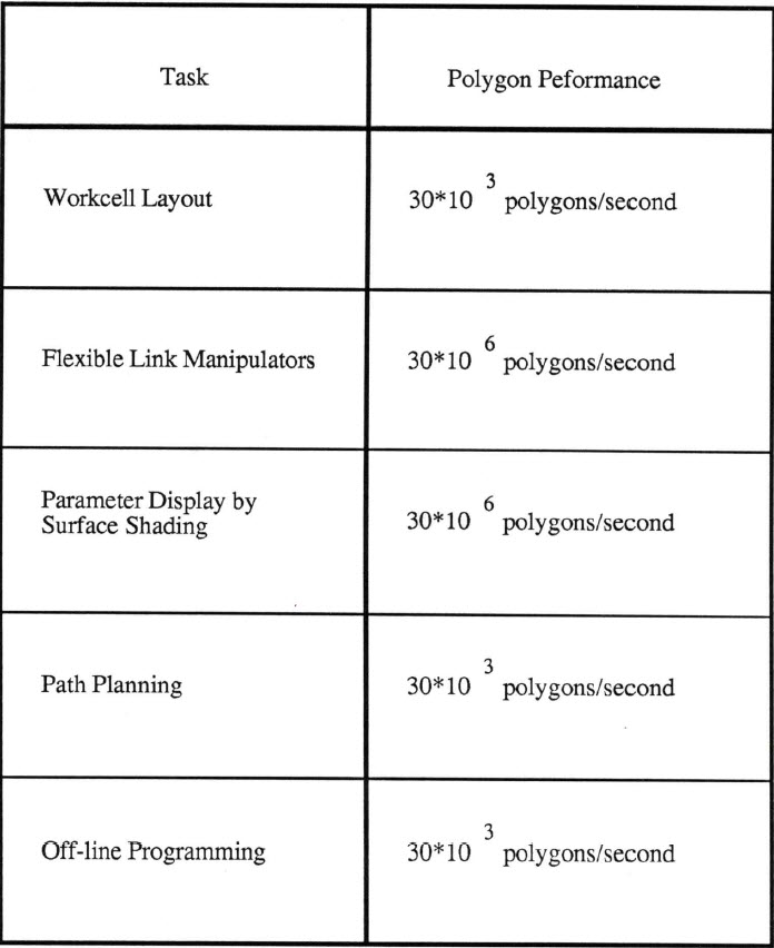
It is necessary to have a surface description in order to present a visual simulation of a three-dimensional object. The conditions at the surface of an object are what actually determine the appearance of the object. An obvious attribute of a surface is its color, or more correctly the color of light the surf ace reflects. Another attribute of a surface is its texture, rough or smooth, etc. A surface can reflect diffuse light, light that is scattered equally in all directions, and it can reflect light directionally. A surface will also reflect ambient light. Ambient light is non-directional light that has typically been scattered by reflections off of other surfaces. A surf ace may even emit light as well as reflect it. A totally complete description of even one surface could be very complex and detailed. In fact, it may be thought of as a modelling problem in and of itself. Animating a typical robot workcell requires that thousands of different surfaces be modelled and displayed many times each second. The result is that the calculation power necessary to do real-time animation of threedimensional solid surfaces with a lighting model is quite large. In order to display a scene with one thousand surf aces at a rate of thirty frames per second requires that the computer display thirty thousand frames per second while performing all of the transformations and modelling that are necessary for each
surface.
30 frames/second * 1000 surfaces/frame = 30000
surfaces/second
This type of processing power is available in current engineering workstations, and as more powerful graphics processing becomes available, higher resolution and more complex scenes may also be animated in real-time.
When viewing an animated scene, some surfaces will be hidden from view as other surfaces pass nearer to the viewer. Showing only the surfaces that the viewer would actually see is called hidden surface removal. Ray tracing is one method that may be used to perform hidden surface removal. Ray tracing techniques follow a straight line from the viewer through the scene, and only the points that the line intersects first are actually shown. Unfortunately ray tracing is computationally expensive because lines must be drawn through every point in the scene after the surfaces have been geometrically
transformed. Z buffering may also be used to perform hidden surface removal. The z buffer is an array of numbers where each number is associated with a pixel on the screen. The numbers kept in the z buffer are the distances between the viewer and each point that will be drawn in the scene. As each new surface is transformed, the distance to the viewer is compared to the value in the z buffer and only the points closest to the viewer are actually drawn. Z buffering is computationally fast but memory-intensive as values must be kept for each pixel on the screen. For example, keeping a z buffer of thirty-two bit numbers for each pixel on a screen that is one thousand by one thousand pixels requires four megabytes of fast access memory.
32 bits/pixel * 1000 x pixels * 1000 y pixels
*4/32 bytes/bit = 4 * 106 bytes
Pipelined computer processing has proven to be of advantage in graphics computers.
This is because many operations must be performed on each point before it can actually be displayed. These operations include geometric transformations and projections, lighting models, surface models and clipping. Specialized hardware that efficiently performs these operations can be arranged in a pipeline where many points can be operated upon at once, with a different operation performed on each one. A computer pipeline might be compared to an automobile assembly line. Many autos are being worked on at once, but different operations are performed at each station. At one station they may be putting on fenders while at another station they are putting on the wheels. The auto is finished after it has been through the entire assembly line.
3.2 ANIMATION METHODS
The animation effect is created by displaying a series of still images in rapid succession with the robot's joint displacements changed by a small amount in each image. The proper values for the joint displacements can be made available to the animation in many ways. An easy way to make the joint displacements available to the animation is to simply calculate them within the same program that is driving the animation. Another method which may be used creates a shared memory structure that may be accessed by both the graphics process and the process that is generating the joint angles. It is also possible to generate the joint angles on a separate computer and then pass the joint angles to the animation computer via a network.
|
|
|
Table 3.1: Required graphics performance for a typical scene animated at a rate of thirty frames per second.
|
For applications that do not require real-time
operation, the joint angles may simply be written to a datafile for
animation at a later time.
|
|
|
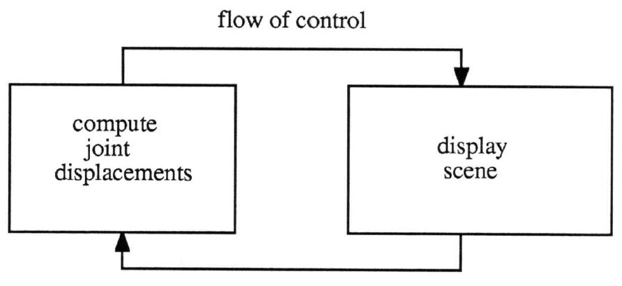
Figure 3. 1: Simple animation loop
|
The joint angles may be calculated within the same program that is generating the animation. The structure for this type of animation is a simple loop. The performance is limited because each block must finish before the other one can start. This structure also limits the modularity of the program because the animation is bound to the kinematics.
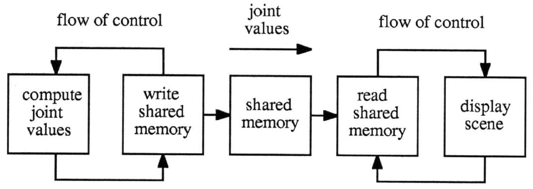
A shared memory structure may be used to communicate joint angles to the animation program. This method is only available with operating systems that support multitasking or multiprocessing. A shared memory is a memory segment that has been mapped into more than one process. For the animation of the robotic system the memory segment is shared by the animation program and the inverse kinematics and decision making routines that are generating the joint displacements. This arrangement may be represented as two loops.
|
|
|
Figure 3. 2: Animation from shared memory
|
The shared memory allows the inverse kinematics and decision making algorithms to be uncoupled from the animation. Changes can be made to one without having to recompile or relink the other. Allocation of the computer's resources can be left up to the operating system or some priority based scheduling hierarchy might be developed to optimize sharing of the computer's resources. It is important to be sure that both processes do not access the shared resources simultaneously. This conflict may be automatically resolved by the operating system or a semaphore or some other technique may be used. The semaphore gets its name from the railroads where a semaphore is used to prevent two trains from colliding on a shared length of track.
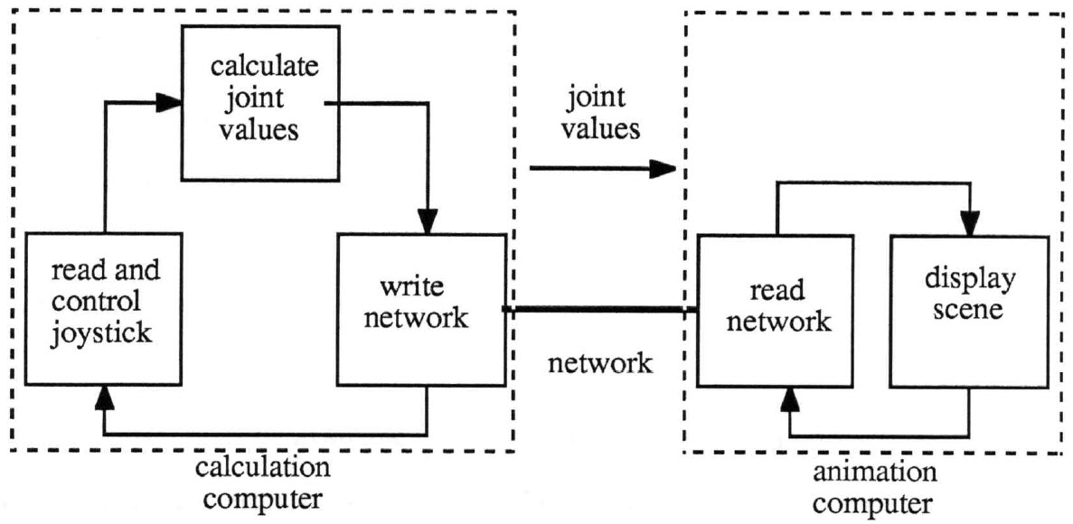
Multiple computers may also be used in the animation. A possible scenario would be for one computer to communicate with a manual controller and generate joint angles while another computer concentrates on generating the graphical images.
|
|
|
Figure 3.3 Animation with distributed computer
processing
|
The network that connects the computers must be considered. A twenty degree of freedom robot whose joint angles are represented as thirty-two bit floating point numbers requires at least six hundred and forty bits of data to specify the kinematic state of the robot for a single frame. An animation loop rate of thirty frames per second requires a network bit rate of at least nineteen thousand two hundred bits per second.
20 DOF/frame * 32 bits/dof * 30 frames/second =
19200 bits/second
This is higher than the bit rate for current RS-232 serial ports, but easily attainable by many other network protocols.
The animation may also be created by cycling the display through a series of preprogrammed positions. The data that specifies these positions may
be stored in data files. The data files may be written in a standard format by inverse kinematics and decision making algorithms, dynamic simulations or by any other robotics research applications where an animated display may be of value, but real-time performance is not necessary.
3.3 SURFACE MATH
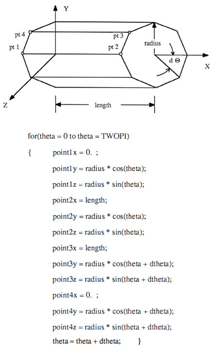
Most currently available digital graphics computers use polygonal representation to display solid surfaces. Polygonal representation describes solid surfaces as filled planar areas bounded by points at the vertices. The minimum number of points that can describe a solid surface is three, a triangle. Lighting models often need to know the direction of the surf ace normal as well as the position of each vertex. Simple geometric relations and computer algorithms can be used to generate the vertex points and the surf ace normals. Actual curved surfaces, such as a pipe, tend to have a continuous curvature. Polygonal representation can only approximate these continuous curves as many flat surf aces. The more flat surf aces that are used, the closer the approximation comes to a continuous curve. Eventually, the resolution of the display terminal is surpassed and there becomes no visible difference between a continuous curve and a polygonal approximation. An algorithm for defining an open tube gives an example of a polygonal approximation of a continuous curve. This example shows the tube as being comprised of many rectangles. The definition of each rectangle requires four points each with x, y and z coordinates.
|
|
|
Figure 3.4: Polygonal approximation of a tube
|
Similar software functions can be written to generate many
three-dimensional shapes. These shapes include boxes, wedges, tubes, cones, spheres and toroids. These functions can be written to have simple scaling arguments such as diameter, length, height and others in order to create a
three-dimensional solid surface graphics library. Translational and rotational transformations can then be used to build more complex objects from the simple functions in the library.
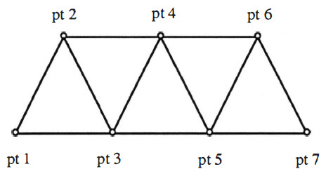
Surfaces that are not easily described by simple primitives can be approximated with triangular meshes. Sets of points on the surface are identified and triangles are then drawn between the points. Triangles offer the finest resolution because three points is the minimum to describe a surface. There is also a computational benefit associated with using triangular meshes.
This is because computer graphics typically involves many transformations and operations on each point that is to be displayed. Since two points on each triangle in the mesh also specify two points on an adjacent triangle, the computer only has to transform one new point for each new triangle.
|
|
|
Figure 3.4: Triangular mesh
|
As an example, consider a mesh of five triangles. In order to draw the first triangle, 123, points one two and three must be transformed. However, in order to draw triangle 234, only point four now needs to be transformed since points two and three have already been transformed. This type of pattern continues through the mesh. The benefits in computational performance result from the fact that fewer points need to be transformed.
Splines can also be used to approximate curved surf aces. Splines typically maintain continuity of position, slope and the rate of change of slope to approximate a continuous curve.
A lighting model enhances the realism of solid surface computer graphics. A lighting model may use the color, location and orientation of the light source; the surface properties, location and orientation of the surface and the position and orientation of the viewer in order to determine the shading of each point on the surface. Lighting models can be extremely complex. Typical lighting in the real world may come from infinite light sources, such as the sun where light rays may be considered to be parallel, from local lights that diverge and from ambient light that has been reflected and scattered by many other surfaces. The best performance is typically obtained with a single infinite light source. Since the light from an infinite source is parallel, the lighting vector remains constant throughout the scene. Lighting models may also incorporate the surface normal at each vertex. Polygonal graphics that specify surface normals that are actually normal to the surface tend to appear faceted with
distinct color changes between polygon faces. The surf ace normal may also be specified as an average between the two polygons to give smoother shading.
Generating the polygonal representation typically involves computer algorithms that sweep through some type of geometric relation. Performing these calculations for each display frame represents a computational load. Significant performance benefits can be obtained if these calculations are performed only once and the results stored in fast access memory. The animation algorithms then read the points and normals out of memory without having to recalculate them each time. This results in faster graphics, but the computer code becomes more complicated because a fast access database must be built to include the surface description of all objects in the scene.
3.4 FEATURE BASED MODEL
There may be other features associated with the model in addition to the information necessary to produce the actual visible display. The range of motion possible for each joint should be accounted for in an animated simulation. The forward kinematics is a feature that is associated with the animated display. Dynamic features may also be associated with the model.
Joint limits are an excellent example of the need to specify the robot model as completely and accurately as possible. If the joint limits are not accounted for in the model, then it may be possible to have the animation appear to be fine while the actual robot has reached a physical joint limit. Attempting to drive the joint past the limit could damage the robot. Joint limits may be
incorporated into the animation model at the modular level. Visible warnings can be given when the joint limits are reached.
Forward kinematics is another feature that may be incorporated into the animation of robotic systems. By incorporating the forward kinematics as a feature of the model, the state of the robot for each frame is determined by the value of the joint variables. This is similar to an actual robot where, neglecting compliance, the visible state of the robot is determined by the angles at the revolutes and the lengths of the sliders. The forward kinematics for the animation is determined by the topology and content of the system, in other words, which types of joints are present and how they are connected. The topology remains constant while the values of the joint variables is changed to produce the animation effect.
It is also possible to associate dynamic features with the animation. The addition of dynamic features would result in a much more complex model, because the topology of the system and the values of the joint variables no longer completely specify the state of the robot. Deformations would cause the appearance of the display to change; for instance links might bend and oscillations could develop. Information about the dynamic state of the robot might be conveyed to the viewer through surf ace shading and coloring. A dynamic model that includes compliances, damping and mass content could be used to create an animation that receives joint torques and external loads as input rather than simply joint displacements. The correctness of the animation would then be dependent upon the accuracy of the dynamic model.
3.5 Precision
In many respects the computer animation of robotic systems is an instrumentation application. There is a transduction process where numerical information is translated into visual information that is used to evaluate the system state and performance. As with most instrumentation problems, the question of precision is of extreme importance. The precision, as well as the resolution and range of the animation, should be examined. The animation instrument has two distinct parts: the numerical representation and algorithms that drive the display and the display terminal itself.
The precision of an instrument is the number of distinguishable different states the output may assume. For the case of an object on a computer screen, a reference point on the surface of the object might occupy any of the pixels on the screen. Current graphics computers have on the order of one thousand by one thousand, or one million different pixels that the reference point may occupy. The precision of the computer algorithms depends upon the internal numerical representation. In the case of floating point numbers that are represented by one sign bit, seven bits of exponent and a twenty-four bit mantissa, the precision is twenty-four bits or seven decimal digits. Round-off and truncation error can also affect the numerical precision, however if the numerical precision is a problem, higher precision numerical representation can be used. Thus it is seen that the limiting factor of the precision of the animation is the display terminal.
The range of the instrument is the difference between the minimum output state and the maximum output state. The range of a terminal that has one thousand pixels on each axis is simply one thousand pixels in the horizontal and vertical directions. The range of the numerical representation again depends upon the specific type of numbers that are used for the computation. Citing the example of a floating point number with one sign bit, seven exponent bits and a twenty-four bit mantissa, the range is from 2. 7 *
10-20 to 9. 2 * 1028 and zero.
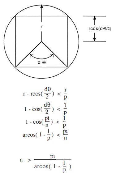
The resolution of an instrument is the smallest change in input that will result in a predictable change in the output. The output of the computer animation of a robot is a visual image of the robot, and the input is the value of all of the joint variables. The resolution of the animation is the smallest change in the value of a joint variable that can be reliably seen on the display. Complicating the resolution of the display is the possibility of mapping different scales of dimensions onto the computer screen. Assuming, for instance, that a robotic workcell that is three meters on each edge is mapped onto a display terminal that is one thousand pixels on each axis, then the resolution is three millimeters. The resolution could be increased by mapping a smaller portion of the workcell onto the computer screen, however this would decrease the range of view. The resolution of the numerical representation of the robot within the computer is highly dependent upon the algorithms that are used to generate the surface description. When using polygonal representation, the number of flat sides used to approximate a curved surface is an important consideration. Consider a tube of radius r with n flat sides. The radius covers some number of pixels, p. The distance between each pixel is therefore rip . It is possible to calculate the number of flat sides that the object must have so that the polygonal representation is not within the resolution of the screen. The difference between the actual radius and the polygonal approximation of the radius must be less than the resolution, r/p.
|
|
|
Figure 3. 6: Polygonal approximation of a circle |
|